How TeselaDB performance is measured

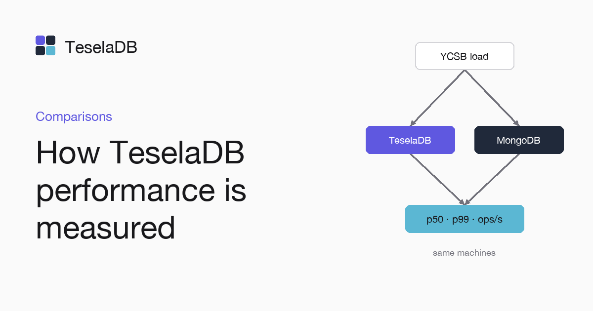
TeselaDB does not publish performance figures without their method. What follows explains how they will be measured, with which tool, which loads and which rules, so that you can judge each result when it comes out and repeat it on your own machines. Until then, the performance page shows no numbers at all.

The tool

Every measurement comes from teseladb-bench, a program in the same repository as TeselaDB. Each measurement is a named scenario, and with --target the same scenario runs against TeselaDB or against MongoDB through a client of its own for the MongoDB protocol, so both systems get the same operations. With an https:// address, the rest scenario measures the REST API.

cargo run -p teseladb-bench --release -- --scenario ycsb-a --target mongodb://127.0.0.1:27017 \
  --warmup 10s --duration 60s --concurrency 64 --json ycsb-a.json

The command above runs YCSB A against the server in --target. It first warms up for ten seconds, then measures for a minute with 64 operations in flight and leaves the report in JSON.

The loads

The main loads are YCSB A to F, as published. They use records of ten fields of 100 bytes and the three distributions of the standard: zipfian, uniform and "latest". Each letter changes the ratio between reads and writes, and YCSB E adds range scans, so that together they cover from an almost read-only load to one that reads and writes the same record.

There are also two scenarios of its own. cores-curve repeats YCSB A, B and C with 1, 2, 4 cores and so on up to the maximum you set with --max-cores, and draws how throughput grows as cores are added. disk-usage measures the bytes each document takes on disk against an encoding that stores metadata in every field.

How a measurement runs

Each scenario has its warm-up, its duration and its concurrency, and it can run in an open loop at a fixed rate of operations per second, with --rate. The difference shows in the high latencies. In a closed loop, a client waiting for a slow answer stops sending, the load drops right when the server struggles and the high latencies vanish from the measurement. At a fixed rate, requests keep arriving and the queue shows.

Each measurement keeps latency histograms with the p50, p99 and p99.9 percentiles, and writes its report in text and in JSON. That JSON is also the baseline. With --baseline, a run is compared with an earlier one and fails if p50 or p99 get worse by more than 10 %, so a performance regression is caught like a failing test.

The same machines

TeselaDB and MongoDB Community run on the same machines and with the same load. Each TeselaDB core thread is pinned to a CPU and reserves its memory on its NUMA node, and each comparison is published with the machine's fingerprint and the versions of both systems, so anyone can tell on which hardware each number came out.

What is compared

YCSB A to F is measured on three nodes. The comparisons with MongoDB repeat YCSB A, B and F with 3 and with 9 nodes. They include sustained inserts with ObjectId as key. They also measure a SIGKILL of the node with the most leaders, with the time to the next confirmed write and the share of operations that fail. Linearizable reads by _id are compared with readConcern: "linearizable", and so is a query on an indexed field that is not the shard key, with the nodes it touches and its latency. Adding a node to a 100 GB cluster is measured too.

There is a less obvious comparison. In TeselaDB each node leads some ranges and follows others, so it spreads across all of them the work that a single primary does in a replica set. To know how much that gains, the F/L ratio is measured: F is the CPU cost of applying a write on a replica and L the cost of coordinating it on the leader. Both are measured with a search index and without one. With R replicas, write capacity comes out as C·R / (L + (R−1)·F) against C / L for a single primary, where C is the CPU capacity of one node. If applying costs much less than coordinating, spreading leaders multiplies capacity; if it costs nearly the same, the gain is small. Only the measurement will say which case is the real one.

Search is compared with MongoDB Community and mongot, in latency and in the time until a write appears in the results. For $vectorSearch, latency and recall@10 are measured with the same numCandidates on both systems, because a faster vector search that finds fewer correct neighbours is not an improvement.

When you will see figures

The results will appear on the performance page with their method and the machines' fingerprint. Each number will come with its scenario and its options, so you can run the same teseladb-bench command against your own cluster and compare.